If you are not satisfied with the Google Forms built-in tool for analyzing responses, you can select google spreadsheet as a response destination and analyze the data there.
It is very easy if you have a Form that is like a survey, you collect all the responses at once and then do the analyses. You have all the responses, you can select what to copy and paste and then you can create graphs or do some extra calculation.
But if your Form acts as a data entry point, like when you collect daily sales or get data periodically, then you have a problem. You can copy and paste the current data from the responses and do the necessary analysis, but when the new responses come in you have to do the whole procedure again.
So now, in order to be able to create a graph or maybe a special report that will always include the latest responses, you have to use functions that can pull and filter the data.
Google form to spreadsheet
Google can send the responses from the Google Form to a spreadsheet. Once you connect the Form to a spreadsheet, the responses are sent automatically to the spreadsheet after form submission.
To connect a spreadsheet to your Form, go to the “Responses” tab on your form and click on the spreadsheet icon, or you can click on the “Select response destination” option from the three-dot menu.
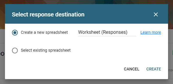
Now, to access the spreadsheet just click on the spreadsheet icon from the responses tab.
When a new spreadsheet is created, Google Forms will name the first sheet as “Form Responses 1”. This sheet will collect all the responses from the connected form and you should not change anything there if you expect more responses.
Note: You can change the name of “Form Responses 1” sheet to something shorter and without blanks in order to make the formulas more readable.
To make Google Forms Spreadsheet Data Analysis on the responses you need to create a second sheet and add all the formulas there. In that new sheet, you can add formulas to pull all or specific data from the “Form responses1”, add graphs and do an extra calculation.
The first problem that you will have is to correctly reference the data from the Form Responses sheet because when the new data comes from the form it adds a row in your sheet. A lot of people make a mistake and reference a set of cells instead of referencing the whole column or columns. So, to get a specific data from the Form Responses sheet you better reference the whole column and filter out the values you need. Before we continue with the formulas we better know how to:
Reference whole column in a sheet
To use formulas to analyze an unknown range of cells, first, you have to learn how to reference a whole column (infinite number of rows in a column) and not only one or a limited number of cells.
To reference a cell in the function we use, for example, the expression A1 and to reference a limited number of cells or a range of cells, we use the expression A1:A10. And you are going to make a mistake If you think that you can reference all the cells in your column A with the expression A1:A1000 (1000 is the number of rows in that sheet) because every time the form is submitted it adds a new row in your sheet.
So, to always include all the entered data, let’s say in column “A”, use the expression A1:A or the expression A1:B to reference two columns (A and B) and so on.
Using this type of reference you can easily pull all or a part of the data from the response sheet and do extra calculations or analysis.
Analyze data from response sheet
There a lot of formulas that work with a range of cells like, for example, functions SUM, MAX, MIN, COUNTIF and so on. If we use them in our sheet we can do a basic calculation on the responses, as we can see in the next example:
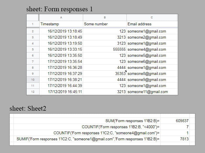
The responses collected with a Google Form are in the sheet ‘Form Responses 1’. As you can see, I have created a new sheet ‘Sheet2’ and add the formulas there, referencing the cells from the responses sheet using the expression ‘Form responses 1’!B2:B (how to Reference data from other sheets).
In the first formula, SUM(‘Form responses 1’!B2:B), I calculate the sum of all the values from the B column in the sheet ‘Form responses 1’. By using the expression ‘Form responses 1’!B2:B this formula will always include all the new entries in the calculation.
In the formulas that use COUNTIF I do the same reference and count the cells that meet the criteria.
In the last formula, SUMIF(‘Form responses 1’!C2:C, “someone1@gmail.com”, ‘Form responses 1’!B2:B), I sum the numbers in the range ‘Form responses 1’!B2:B that meet the criteria specified in the formula.
This means that the formula will go row by row and compare the value of each cell in the first range ‘Form responses 1’!C2:C if they are equal to the string “someone1@gmail.com”. If the criteria is met it will include the corresponding cell from the second range ‘Form responses 1’!B2:B. By examining the response sheet, we can conclude that this formula will include only the rows 2, 4, 8 and 11, and will calculate only the numbers from that rows contained in column B.
Now, this is very easy, but the real problem is when you try to use a more complex formula. What I mean by more complex is that the formula includes more than one function in it or the function itself doesn’t support ranges, like this one:
COUNTIF ( DAY('Form responses 1'!A2:A), "=16")We know that COUNTIF function can work with a range of cells, but DAY function is not build to do that.
A short reminder, DAY function will return the day of the month from the specific date, in this case, from column B, you can read more here: DAY function.
What this formula is intended to do is basically count how many responses are entered on the 16th day. I say intended because is not going to work, the DAY function cannot process a range of cells and here is the result in the sheets:

Using arrayformula for non-array functions
In order for the previous formula to work, I must use the function ARRAYFORMULA that will make the non-array functions to use arrays. This function will make the function DAY to use the range by making an array of formulas.
For the formula to work we are going to put everything in the ARRAYFORMULA function like this:
=ARRAYFORMULA( COUNTIF ( DAY('Form responses 1'!A2:A), "=16") )Here is the result from the formula:
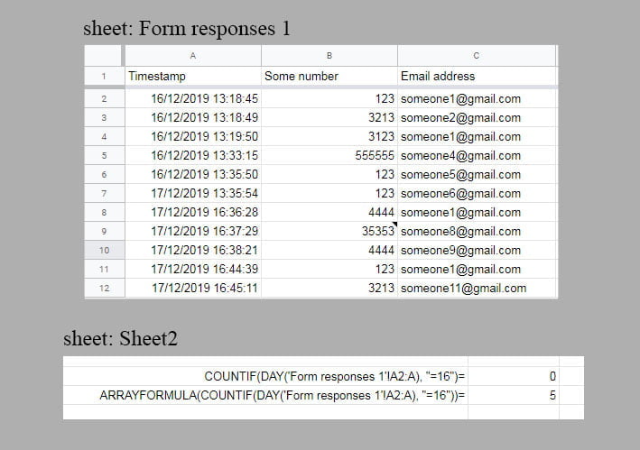
This is not the only use of ARRAYFORMULA function, it can also get a range of cells. Look what happens if you use this function with a function that doesn’t handle a range of cells, like function DAY.
=ARRAYFORMULA( DAY('Form responses 1'!A2:A) )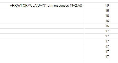
As we can see from the example, we can get a list of values using ARRAYFORMULA with any function. So now, I can return a list of values based on some criteria.
Let’s say I want to get all the e-mails from the responders that submitted their answer on the 16th. For this, I’m going to use the IF function:
=ARRAYFORMULA( IF( DAY( 'Form responses 1'!A2:A)=16,'Form responses 1'!C2:C,))
This formula will compare the responses timestamp (column A) if they are equal to 16 and if they are it will display the e-mails from the C column.
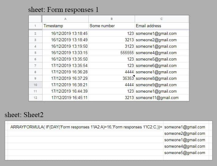
While this type of formulas is useful for making calculations, they are not good to display a list of data from the responses sheet. The previous formula filtered a set of data that is consecutive, but if the data is spread across the sheet it will be a problem to display the results. Let’s adjust the formula to display the data based on the respondent’s e-mail. The formula will look like this:
=ARRAYFORMULA( IF( 'Form responses 1'!C2:C="someone1@gmail.com", 'Form responses 1'!B2:C, ))
Here is the result of that formula:

Note: In this example, we display data from two columns with the expression ‘Form responses 1’!B2:C
Аlthough, the result from the formula is OK, the way it is displayed is a problem, returning the values that did not match as empty rows.
So, to avoid this, there is another solution to display filtered data from the responses sheet using QUERY or FILTER functions. Even though the QUERY function can perform more complex calculations, I’m not going to use it here. I’m going to talk about:
How to use FILTER function
The FILTER function acts the same as the filter options in your spreadsheet. So, basically it will filter the data based on values in one or more columns. Here is the syntax for the FILTER function:
FILTER( range, condition1, [condition2, …])
The range is the data that is going to be displayed if the condition is met. This means that if the condition is met in the corresponding row it will display the data specified in the range. You have to specify at least one condition and the length must be the same as the range.
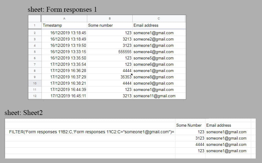
Now, in order to recreate the previous formula with the FILTER function we are going to use the next expression:
=FILTER( 'Form responses 1'!B2:C, 'Form responses 1'!C2:C = "someone1@gmail.com")
Where ‘Form responses 1’!B2:C is the range to be displayed if the condition ‘Form responses 1’!C2:C = “someone1@gmail.com” is met.
And here is the result:
Filter function to analyze data from Google Forms
As you can see from the example, it displays the data without blank rows.
You can use FILTER function with more conditions specified and get more specific lists. Also, you can use the results from the function to do an extra calculation. Like for example, the next formula is going to sum the numbers entered in the “Some Number” field submitted only from “someone1@gmail.com”
From here on, you can create graphs and publish your data on Google Sites and create a fully automated system. For example, you can create a Google Form that will collect daily sales info and you can filter the data and display a daily, weekly or monthly sales report. For this, I plan to create a how-to guide, so check the blog regularly for any updates.
Here is the link for the spreadsheet that I used in this how-to: The Google Spreadsheet
If you have any questions just post a comment I’ll get back to you.
