
If you’re looking beyond the built-in analytics in Google Forms, you’ve probably turned to Google Sheets for deeper data analysis. It’s the perfect next step.
For a one-time survey, the process is simple: you collect all the responses, copy the data, and then create your graphs and calculations. But what happens when your Form is an ongoing data entry point, like for daily sales logs or periodic reports? Copying and pasting the data every time a new response comes in is tedious and inefficient.
The real goal is to create a report or graph that updates automatically with every new submission. To do that, you need to use functions that can dynamically pull and filter your live data. This guide will show you how.
Note: Check the example spreadsheet for referenced formulas, link at the end of the article
Step 1: Connect Your Google Form to a Spreadsheet
First, you need to send your Form responses to a Google Sheet.
- In your Google Form, navigate to the “Responses” tab.
- Click the green spreadsheet icon. You can also click the three-dot menu and select “Select response destination.”
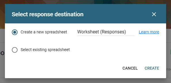
This creates a live link. All new submissions will now automatically appear in this spreadsheet. The sheet where responses land is typically named "Form Responses 1" by default.
Pro Tip: You can rename the "Form Responses 1" sheet to something shorter and without spaces (like “Data”). This will make your formulas cleaner and easier to read later on. For your analysis, always create a second, separate sheet. This keeps your raw data pristine while you build your reports.
The Golden Rule: How to Reference a Full Column
One of the first hurdles you’ll encounter is referencing your data correctly. When a new form is submitted, Google adds a new row to the sheet.
Many people make the mistake of referencing a fixed range, like A1:A1000. But what happens when you get your 1001st response? The formula breaks.
To ensure you always include all current and future data, reference the entire column.
- To reference all of column A (starting from A1), use:
A1:A - To reference all of columns A and B, use:
A1:B
Using this “open-ended” reference style is the key to creating a fully automated analysis.
Basic Analysis with SUM, COUNTIF, and SUMIF
Let’s start with some foundational formulas. In your new analysis sheet, you can pull data from your response sheet (let’s call it 'Form Responses 1').
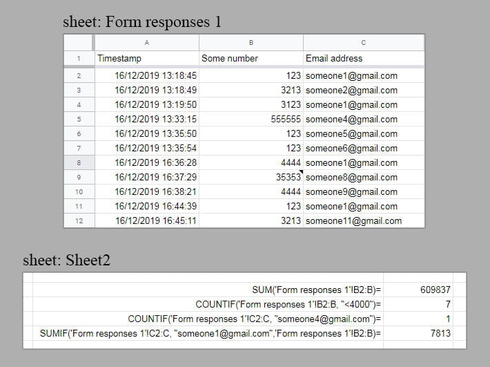
Imagine your response sheet has a column of numbers (Column B) and a column of emails (Column C). Here’s how you can analyze it:
- To sum all numbers in Column B:
=SUM('Form Responses 1'!B2:B)This formula will automatically include new entries as they arrive. - To count specific entries with
COUNTIF:=COUNTIF('Form Responses 1'!C2:C, "someone1@gmail.com") - To sum numbers based on a condition with
SUMIF: This formula sums the numbers in Column B, but only for rows where the email in Column C is “someone1@gmail.com”.=SUMIF('Form Responses 1'!C2:C, "someone1@gmail.com", 'Form Responses 1'!B2:B)
Unlocking Superpowers with ARRAYFORMULA
Now for a more complex problem. What if you want to perform a calculation on a whole range of cells, but the function you’re using (like DAY, MONTH, or YEAR) doesn’t naturally support ranges?
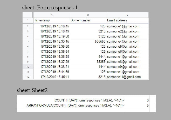
For example, the DAY function extracts the day of the month from a date. If you try to use it with COUNTIF on a whole range, like this, it will fail:
=COUNTIF(DAY('Form Responses 1'!A2:A), "=16") <– This won’t work!
This is where ARRAYFORMULA comes in. It enables non-array functions to work with arrays (or ranges). By wrapping your formula in ARRAYFORMULA, you tell Sheets to process the function for every single row in the range.
- The Correct Way:
=ARRAYFORMULA(COUNTIF(DAY('Form Responses 1'!A2:A), "=16"))This now correctly counts how many responses were submitted on the 16th day of the month.
You can also use ARRAYFORMULA to output a whole list of values. For example, to get a list of emails for every response submitted on the 16th:
=ARRAYFORMULA(IF(DAY('Form Responses 1'!A2:A)=16, 'Form Responses 1'!C2:C, ""))
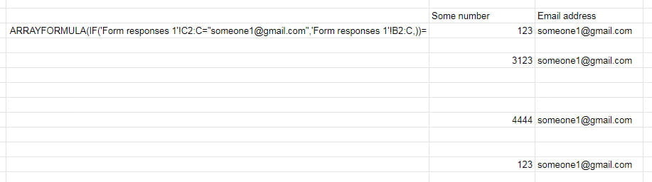
While this works, you’ll notice it leaves blank rows for the data that doesn’t match. It’s functional, but not very clean.
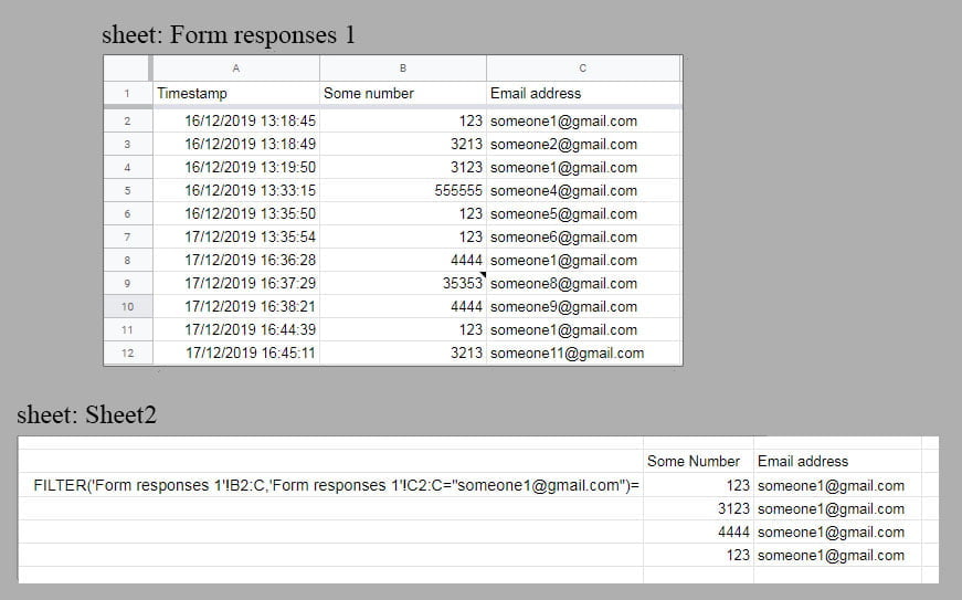
=ARRAYFORMULA( IF( 'Form responses 1'!C2:C="someone1@gmail.com", 'Form responses 1'!B2:C, ))
Here is the result of that formula:
For a better solution, we turn to the FILTER function.
The Cleanest Way to List Data: The FILTER Function
The FILTER function does exactly what its name implies: it filters your data based on a condition and displays only the rows that match—with no blank spaces.
The syntax is: FILTER(range, condition1, [condition2, ...])
range: The data you want to display.condition1: The test to apply to a column. The range for the condition must be the same length as the data range.
To recreate our last example (listing data for a specific email) cleanly, we use:
=FILTER('Form Responses 1'!B2:C, 'Form Responses 1'!C2:C = "someone1@gmail.com")
This formula displays the data from columns B and C only for the rows where the email in column C matches “someone1@gmail.com”. The result is a clean, compact list.
You can even perform calculations on your filtered results. To sum the numbers submitted only by “someone1@gmail.com”:
=SUM(FILTER('Form Responses 1'!B2:B, 'Form Responses 1'!C2:C = "someone1@gmail.com"))
The QUERY Function (The All-in-One Tool)
The QUERY function is the most powerful tool in your arsenal. It uses SQL-like language to let you select, filter, and sort your data.
Let’s say your responses are in a sheet named 'Form Responses 1'. You could use this formula in a new tab to pull a list of everyone from the “Marketing” department:
=QUERY('Form Responses 1'!A:G, "SELECT * WHERE C = 'Marketing'")
'Form Responses 1'!A:Gis the range of your data."SELECT * WHERE C = 'Marketing'"tells the formula to grab all columns (SELECT *) where Column C is exactly “Marketing”.
From here, the possibilities are endless. You can feed these filtered lists into charts, connect them to Google Sites, and build a fully automated reporting system.
Here is the link to the example spreadsheet used in this guide: Google Spreadsheet
If you have any questions, just post a comment, and I’ll get back to you!